For this tutorial, let us assume that we want to map soil silt content over an area but we don’t have direct knowledge on the relationship between soil silt content and environmental conditions. However, we have some field sample points at each of which soil silt content for a given horizon was measured but these samples were not collected based on any rigid sampling designs. SoLIM Solutions now provides a way (referred to as sample-based inference) to map the spatial variation of soil just using field samples which does not need to be collected based on any rigid sample designs. You can certainly use this approach with samples collected based on a well-designed sampling scheme.
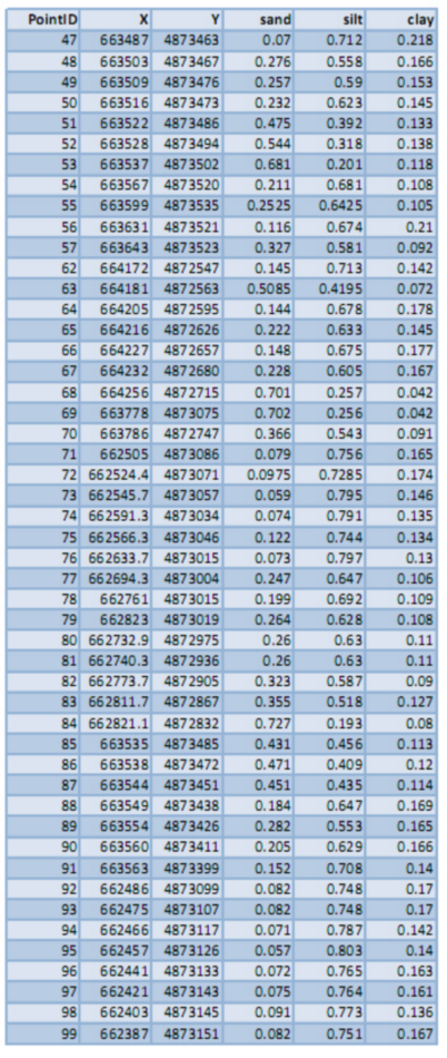
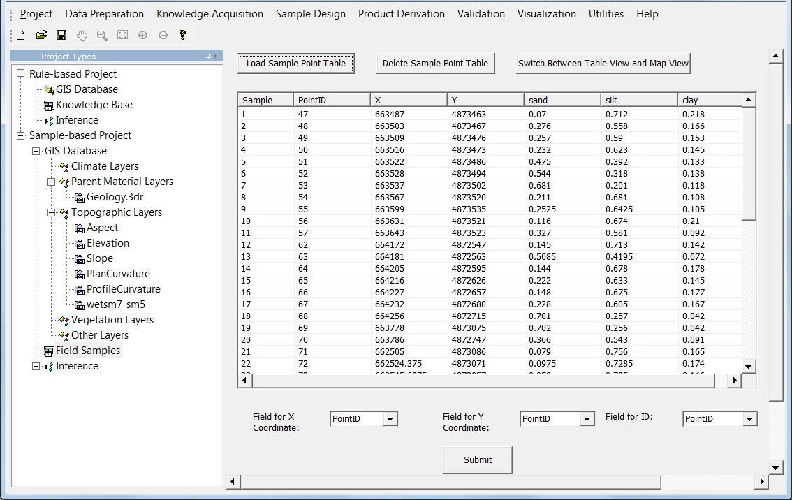
Suppose that the following table is what you have in terms of information about the field samples you have for an area. The X and Y columns contain the x and y coordinates of each sample location. These coordinates should be in the same coordinate system as that of the environmental data layers. Column "silt" contains the soil silt content of a given horizon for each sample location.
We will create a sample-based project to utilize these field sample points to produce a soil silt map for the area.
We need to create a .csv file to store these field samples first, which is completed outside SoLIM Solutions. The easiest way to do this is to enter the field sample data into a spreadsheet and save it as a .csv file. In this tutorial, this step is already done for you. You can see a "field_samples.csv" file in "<SoLIM Solutions installed directory>\Tutorial_Data\Sample_Based" directory.
Create a Blank Sample-based Project:
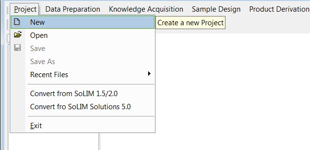
Select "Project->New" to create new project.
Specify Project Name and Project Directory. Here we enter "Test_SampleBased_Project" as the project name and create a new folder "C:\Test_SampleBased_Project" as the project directory.
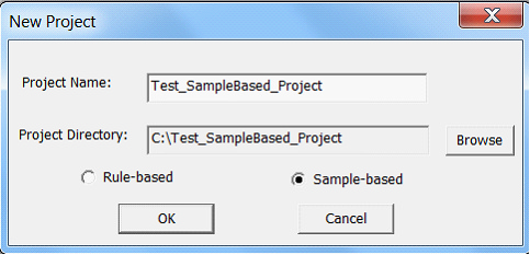
Select "Sample-based" and then click on "OK", a new blank sample-based project will be created for you. The "Sample-based Project" node in the left project panel is activated. In the project directory you just specified, the program generated Test_SampleBased_Project.sip (the project file) and a directory named "GISData" (directory for storing GIS data layers on environment variables) which is currently empty.
Add GIS Data Layers:
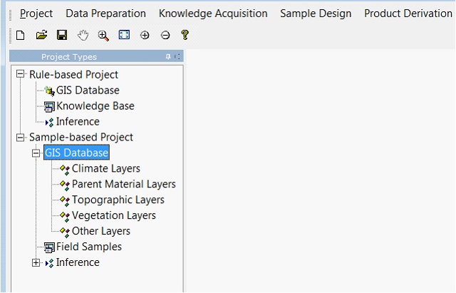
In the left project panel, you will notice that under "GIS Database" node, there are five sub-nodes: Climate Layers, Parent Material Layers, Topographic Layers, Vegetation Layers and Other Layers. We will add our environmental data layers to different sub-nodes.
The native file format for SoLIM Solutions is 3dr format. However, SoLIM Solutions can convert other commonly-used raster file format (e.g. TIFF, ERDAS IMAGE) to .3dr format on the fly. SoLIM Solutions can also rasterize commonly-used vector file format (e.g Shapefile) into 3dr format. See File Converters in the Utilities menu for how.
There are a few data layers in "<SoLIM Solutions installed directory>\Tutorial_Data\Sample_Based" directory. One of them (Geology.3dr) is for parent material. Other data layers are all topographic layers.
Right click on "Parent Material Layers" node. In the pop-up menu, select "Add Layer" to add Geology.3dr to the project.

Similarly, add all the other environmental data layers to "Topographic Layers" node. Note that you can add multiple layers at one time.
The left project panel should now list the data layers you just added. These data layers are also copied to the "GISData" directory in the project directory you specified earlier (here is "C:\Test_SampleBased_Project"). In that way, they become part of the project and can be easily moved around with the project directory.
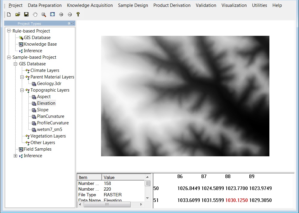
After the data layers are loaded, you can click each layer name in the left project panel to view the layer.
As mentioned earlier, we already have a field_sample.csv file storing all the field sample points. Now we will add it to our project.
Left click "Field Samples" node in the left project panel.
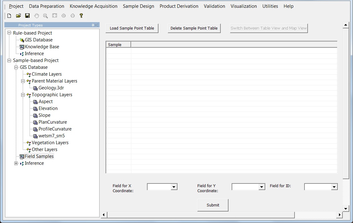
Click "Load Sample Point Table" to add the .csv file to our project.
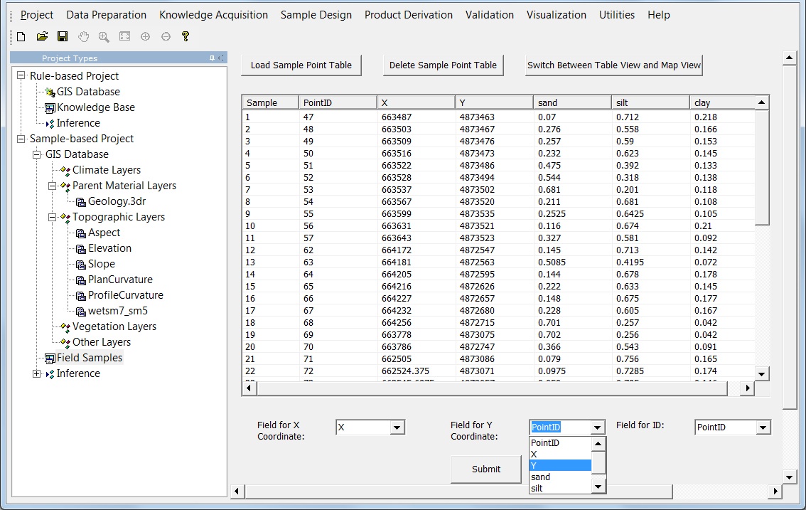
Specify the columns that record X coordinate and Y coordinate by selecting column names from drop down list. Here "X" is for X coordinate and "Y" is for Y coordinate.
Click "Submit", you will see the distribution of the sample points in map view. The red points represent the field sample point in the study area. It should be noted that at least one layer need to be in the GIS Database. Otherwise, you cannot view the distribution in map view. Also, if the coordinates of your sample points are not in the same coordinate system as that of the environmental data layer in the GIS database, you will not be able to see the sample points in the map view.
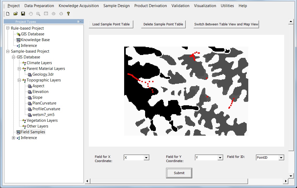
You can always switch to table view by clicking "Switch between table view and map view"
Now we have successfully added field sample points to our project.
Save the Project:
Let's save the project through "Project->Save".
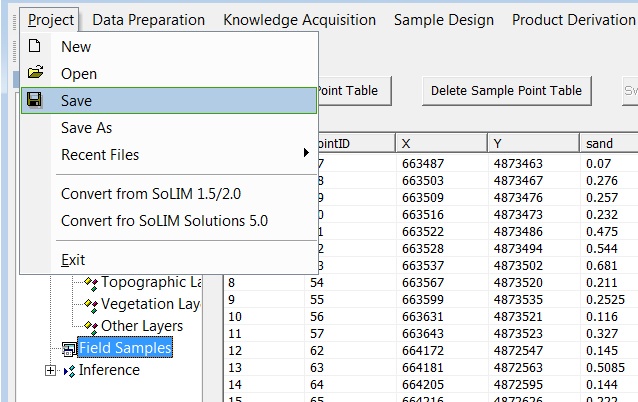
The project configuration and field samples will be saved into "Test_SampleBased_Project.sip" in the project directory.
At this point your project has been created and saved. The next step is to run an inference using the GIS database and field sample points to produce soil silt content map.
Run Inference
SoLIM Solutions can create multiple soil property maps using GIS database and field sample points. In this tutorial, we only infer soil silt content.
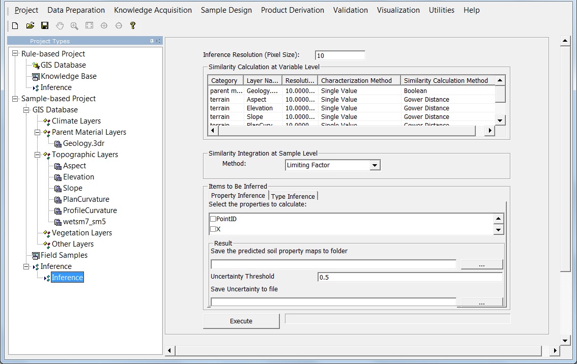
Click "Inference" node to unfold it. Under that node, click "Inference", the view will shift to Inference interface.
Before we make any change to the inference setting, we need understand a few concepts behind sample-based project. The basic idea of sample-based project is to infer soil property/type based on similarity between an unknown position and existing field samples based on the environmental conditions. Therefore, how environmental conditions are characterized and how similarity is calculated are most critical in the inference.
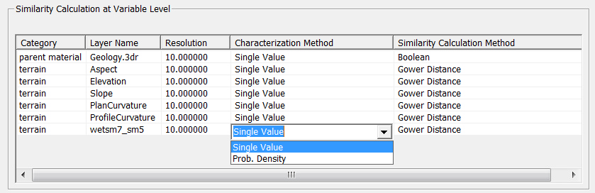
There are two basic characterization methods in this implementation: single value and probability density:
Single value means that the mean value of a given environmental variable over the inference resolution is used in calculation of similarity when the inference resolution (the pixel size) is large than that of the environmental data layer. If the resolutions of the environmental data layers are the same and the inference resolution is also that of the environmental data layers, the single value is simply the original value of the pixel. Probability density means that a probability density function is derived from the values of the pixels over the area of inference pixel when the inference pixel size is greater than the pixel size of the environmental data layer. Probability density method is much more computationally expensive than the single value approach.
Similarity calculation is conducted at two levels: variable level and sample level:
At the variable level, the similarities between an unknown position and sample points are calculated using each environmental layer in GIS database. At the sample level, the similarities derived at the variable level are integrated to yield the final similarity between each unknown position and each sample point.
While you can change the similarity calculation method at both variable level and sample level. In this tutorial, for variable level similarity calculation, we choose "Single Value" as Characterization Method for all environmental layers and we choose "Boolean" as Similarity Calculation Method for Geology layer and "Gower Distance" for all the terrain layers. You can refer to the user manual for the differences of those methods.
Once that is done we need to specify the soil property we want to infer and then run the inference. During the inference process, SoLIM Solutions does not only predict soil property value for every location but also provides the uncertainty associated with the prediction at each location. If the uncertainty is too high (higher than the uncertainty threshold), SoLIM Solutions will assign NoData to that position in the final soil property map.
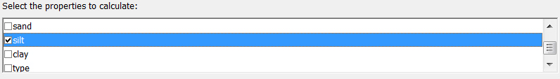
Make sure you are in Property Inference tab. Check the box before "silt".
Click on![]() button within the region of "Inference Result", a dialog will appear for you to create or choose output directory.
button within the region of "Inference Result", a dialog will appear for you to create or choose output directory.
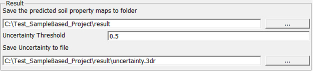
Create a results directory "result" in the "Test_SampleBased_Project" directory to host the output soil silt content map using the "Make New Folder" button.
Click on "OK", the directory will appear on the "Save Result in" text box.
We will use the default uncertainty threshold 0.5.
Click ![]() button to choose the path of uncertainty file.
button to choose the path of uncertainty file.
Click on "Execute", if the inference is finished without an error, a dialog should pop up to inform the completion of the inference. Otherwise, an error message should show up to tell you what was wrong.
Viewing Results:
After the inference has completed, you may want to view the results in graphic form. If you have been following this tutorial so far, you should see "predicted_silt.3dr" file in "C:\Test_SampleBased_Project\result" directory. This file is the final prediction result. You can also find "uncertainty.3dr" file in the project folder.
There are three ways to view the results. One is to convert the 3dr file into GRID ASCII format and view the results in other GIS software, such as ArcGIS (see Untilities->File Converter for details on exporting 3dr file into GRID ASCII format). The second is to use the 3dMapper (available at www.terrainanalytics.com). The third way is to view the results using the Data Viewer provided by SoLIM Solutions 2013. In this tutorial, we will use the 2D Data Viewer to visualize the results.
Choose "Visualization->2D" and open the Data Viewer.
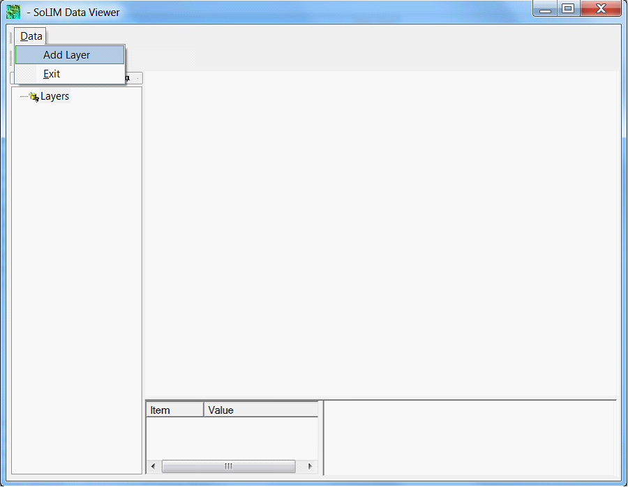
Choose "Data->Add Layer"
Navigate to the output directory and select "predicted_silt.3dr" and "uncertainty.3dr" to open them. You should now see these two data layer are added to the left layer list panel. You can choose one layer to view it the graphic area by clicking the corresponding node in the layer list panel.
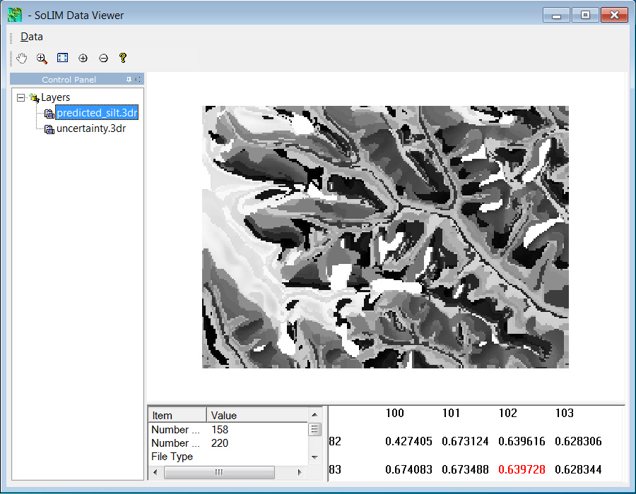
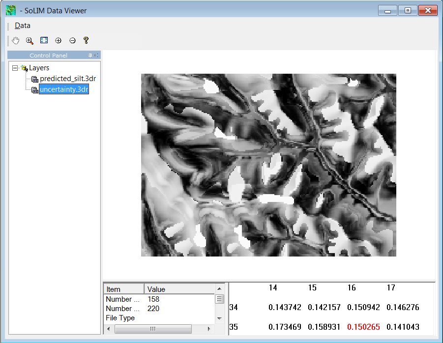
For the soil silt content layer, bright grey represents high silt content and dark grey scale represents low silt content. Note that some pixels have value -9999 which means NoData. This is due to the corresponding uncertainty values at those locations are higher than the uncertainty threshold (0.5 in this tutorial).
For the uncertainty layer, bright grey represents high uncertainty and dark grey represents low uncertainty.