Clearly, with a rule-based project, one is assuming that one has the soil-environment relationships explicitly defined and they can be expressed as rules.
For this tutorial, let us assume that we want to map a soil type (say soil type 1) which occurs under the following conditions:
"South facing slopes with linear planform curvature, sandstone geology (indicated by the number 15 in the geology data layer) and slope gradient greater than 12%". This description of environmental conditions is the knowledge on soil-environment relationship.
Create a Blank Rule-based Project:
Select "Project->New" to create new project.
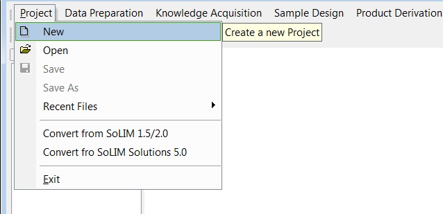
Specify Project Name and Project Directory. Here we enter "Test_RuleBased_Project" as the project name and create a new folder "C:\Test_RuleBased_Project" as the project directory.
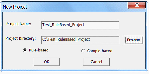
The default project type is rule-based, so we don’t need to make any change. Click on "OK", a new blank rule-based project will be created for you. The Rule-based Project node in the left project panel is activated. In the project directory you just specified, the program generated Test_RuleBased_Project.sip (the project file) and a directory named "GISData" (directory for storing GIS data layers on environment variables) which is currently empty.
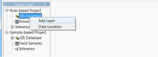
Add GIS Data Layers:
In the left project panel, right click on "GIS Database" under "Rule-based Project" node. In the pop-up menu, select "Add Layer" to add new environmental data layer(s) to the project.
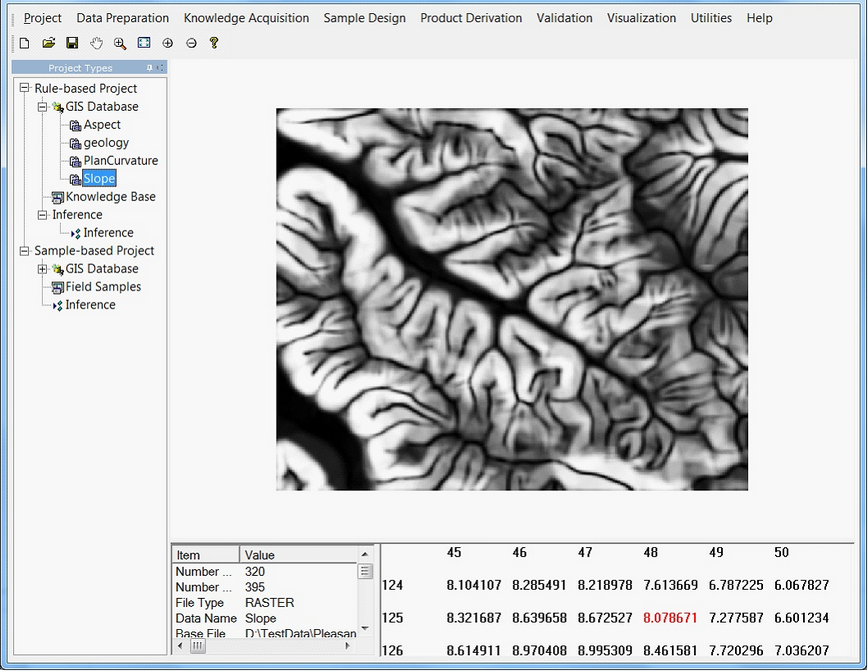
For this tutorial we will add the following four data layers (in 3dr format) from "<SoLIM Solutions installed directory>\Tutorial_Data\Rule_Based" directory: Aspect, Geology, PlanformCurvature, and Slope based on the needed environmental conditions stated in the knowledge stated earlier. You can also include other environmental data layers at this stage which may be needed for mapping other soil types. The native file format for SoLIM Solutions is 3dr format. However, SoLIM Solutions can convert other commonly-used raster file format (e.g. TIFF, ERDAS IMAGE) to .3dr format on the fly. SoLIM Solutions can also rasterize commonly-used vector file format (e.g Shapefile) into 3dr format. See File Converters in the Utilities menu for how.
After selecting the files, click on "Open". The left project panel should now list the data layers you just selected. These data layers are also copied to the "GISData" directory in the project directory you specified earlier (here is "C:\Test_RuleBased_Project"). In that way, they become part of the project and can be easily moved around with the project directory.
After the data layers are loaded, you can click the name of each layer in the left project panel to view the layer.
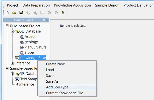
Add Soil Types:
In the left project panel, right click on "Knowledge Base" node and select "Add Soil Type" from the pop-up menu.
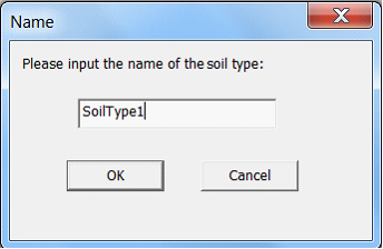
This displays a dialog box for you to specify the name of the soil type. Enter "SoilType1" and click on "OK".
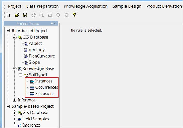
A new soil type is added into the knowledge base. Unfold the soil type node, you will see three sub-nodes are create: Instances, Occurrences, Exclusions. They are used to hold different kinds of knowledge (see Soil Mapping Using SoLIM for discussion on the different kinds of knowledge).
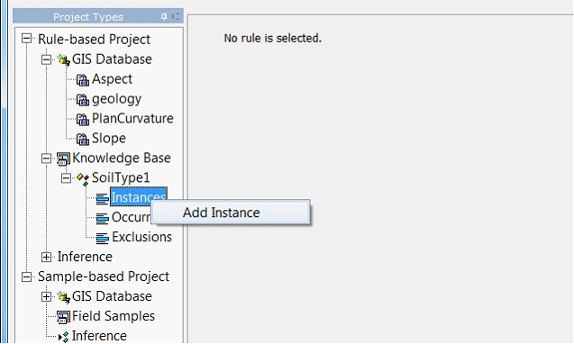
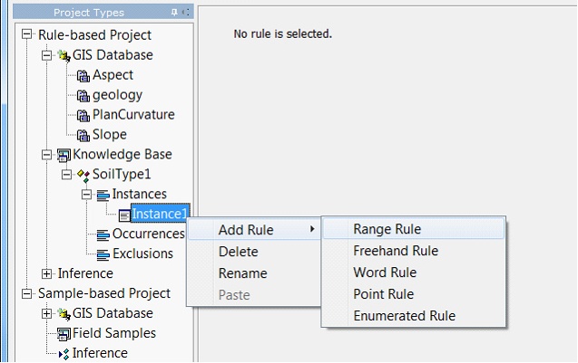
Based on the soil-environment knowledge for soil type 1 ("South facing slopes with linear planform curvature, sandstone geology (indicated by the number 15 in the geology data layer) and slope gradient greater than 12%".) there is only one environmental configuration under which soil type 1 occurs. The environmental configuration takes effect in the whole mapping area, so only one instance is needed to represent the knowledge (global knowledge) in the knowledge base. Right click on the "Instances" node under the "SoilType1" node and select "Add Instance" from the pop-up menu.
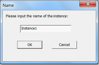
This will display a dialog to let you input the instance name. Enter "Instance1" and click on "OK", a new blank instance will be created.
Under the "Instances" node, you can see the newly-created instance.
Create Rules:
Four environmental variables are used in the soil-environment knowledge for this soil type. Thus, the next task is to create rules for each environmental variable.
Rule for Slope:
We can use range rule to express the knowledge on slope.
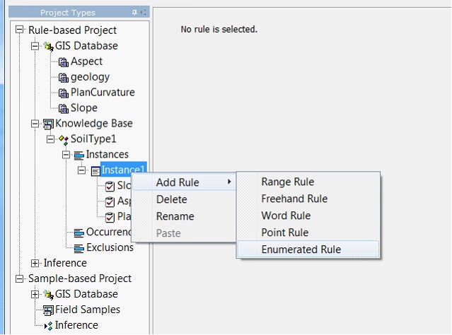
| 1. | Right click on the "Instance1" node. In the pop-up menu, select "Add Rule" and then select "Range Rule". |
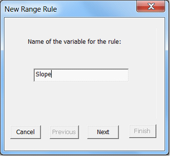
| 2. | Enter the name of the variable for the rule. Here we type in "Slope" then click on "Next". |
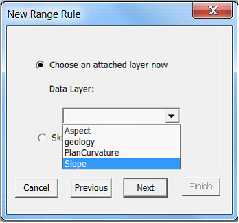
| 3. | Select "Choose an attached layer now", and then select "Slope" from the "Data Layers" drop down list, and then click on "Next". This will allows the inference engine to link the rule defined here with the GIS data layer "Slope" which was defined in the GIS database earlier. |
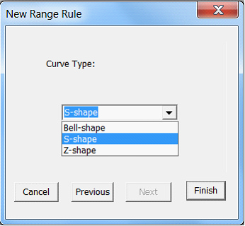
Based on the soil environmental conditions, Soil Type 1 occurs on slopes steeper than 12%. This calls for an S-shaped curve which says that with the increase of slope the membership value for being this soil type also increases (For discussion on curve types see the internet article "Overview of SoLIM" in the Overview of SoLIM section and the Zhu et al., 2013 article in the Representation Scheme section in Appendix D). Click on the "Curve Type" drop down list and select "S-shaped", then click on "Next".
| 4. | Click on "Finish", a default S-shape curve is created for you. The view will switch to rule editing interface. |
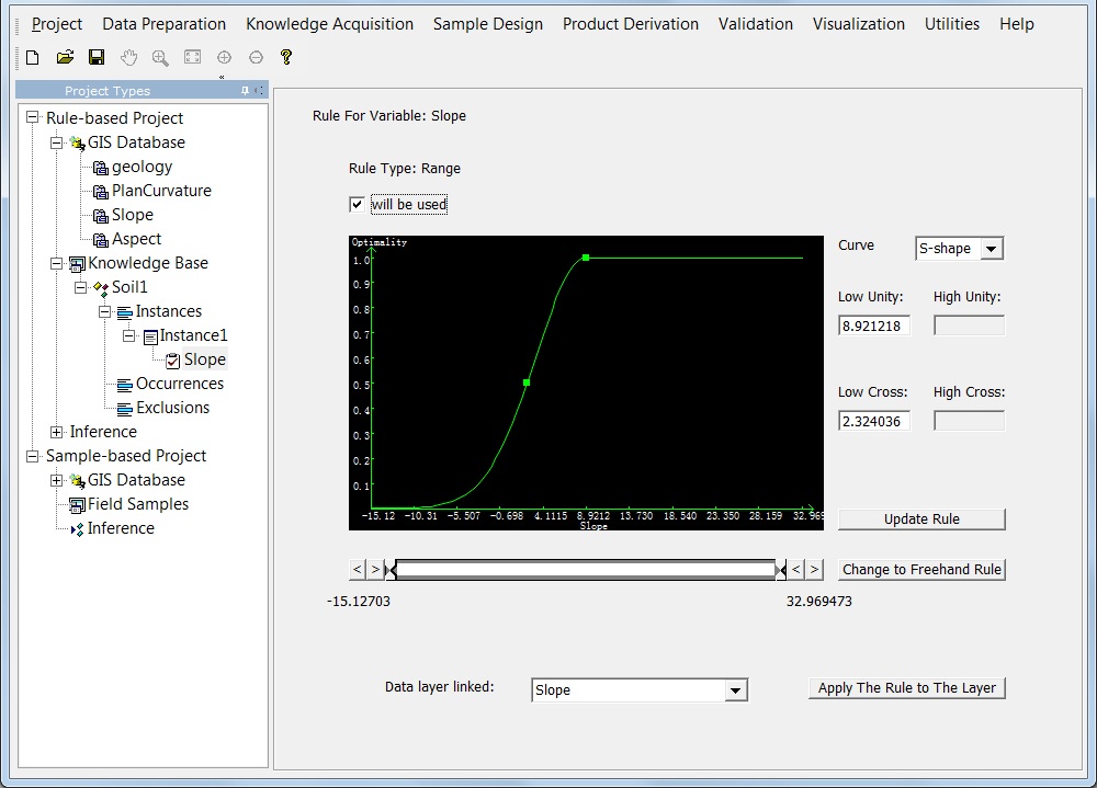
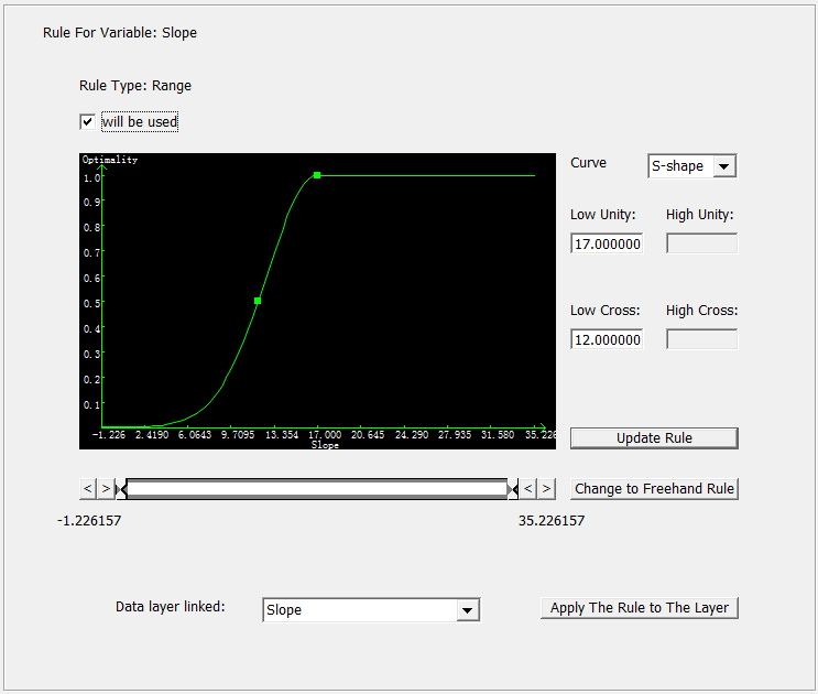
| 5. | We can customize the newly-created rule to better represent the knowledge on slope. The current rule as shown above represents that the soil occurs in areas with slope gradient greater than 2.324%. To make it represent greater than 12%, we need to determine the low unity and low cross. Low unity in this case represents the ideal slope value for the soil to be Soil Type 1. This is another piece of knowledge soil scientists need to provide. Let assume in this case low unity to be 17%. Low cross (the environmental condition at which the membership for this soil type is 0.5) is set to be 12%. When low unity and low cross are all entered, click on "Update Rule" to submit. This brings up the interface shown below: |
You can also click on and drag the green handles (dots) on the curve to adjust the rule. Please try to drag the handles respectively and see their individual impacts on curve and the values in text boxes. You can also click the "Apply The Rule to The Layer" button to see the effect of the rule.
Rule for Aspect:
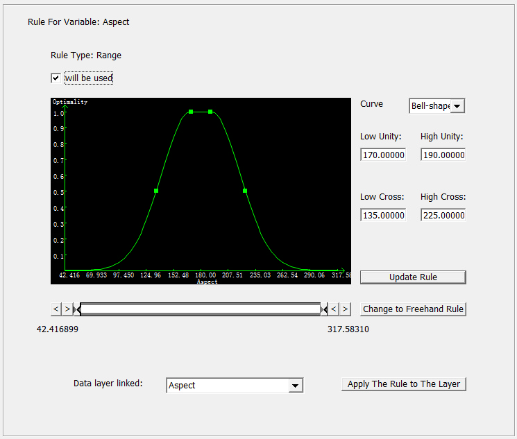
The way to create rule for aspect is much the same as that for slope, except using Bell-shape rather than S-shape curve in the second step. The reason for using the Bell-shape rule here is that the knowledge states that the soil type is on "south facing slope". Thus, the membership value for being "south" should increase first when the slope aspect value increases from 0 and then should decrease when the slope aspect value is over a certain value. When the default rule is created, we should adjust the rule to capture the essence of "South". Absolute "South" means aspect is 180°. We will assume that a range of values around 180° is perfectly suitable for the soil. Thus we will take "South" to mean 170° (low unity) to 190° (high unity). A slightly larger range, from 135° (low cross) to 225° (high cross) will cover less than optimal aspect values. Try to make your aspect rule look like the one shown below. The specific values for low unity, low cross, high unity and high cross are case specific and much of this information is provided by the local experts.
Rule for Planform Curvature:
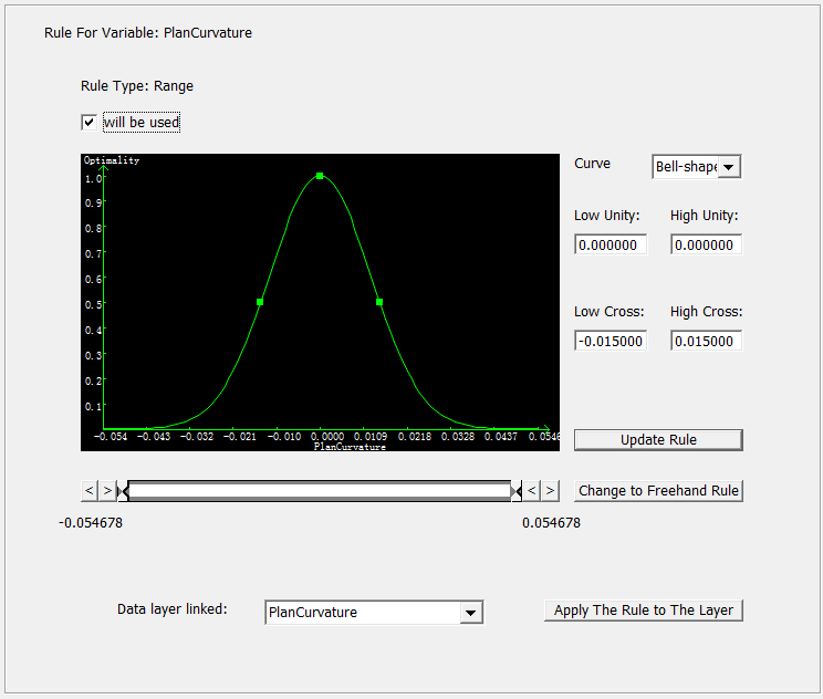
The way to create rule for planform curvature is the same as that for Aspect because linear planform curvature means that the membership value for being linear increases when the planform curvature value approaches zero from the negative and decreases when the planform curvature values deviate from zero into the positive. When adjusting the rule, we set low unity and high unity to 0 to reflect "linearity" (zero curvature) and set low cross and hight cross to --0.015, 0.015 to cover less than optimal planform curvature values.
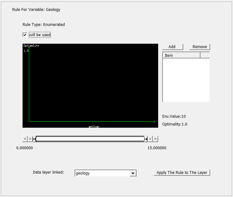
Rule for Geology:
Geology is different from other environmental variables because it is a categorical variable. So you should create an enumerated rule for it. The way to create enumerated rule is very similar to that of creating a range rule.
| 1. | Right click on the "Instance1" node. In the pop-up menu, select "Add Rule" and then select "Enumerated Rule". |
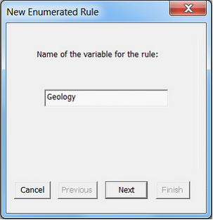
| 2. | Enter the name of the rule. |
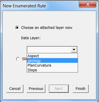
| 3. | Check "Choose an attached layer now", and then select "geology" in the drop down list. |
| 4. | Click on "Finish", a blank enumerated rule will be created for you. The view will switch to rule editing interface. |
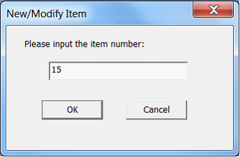
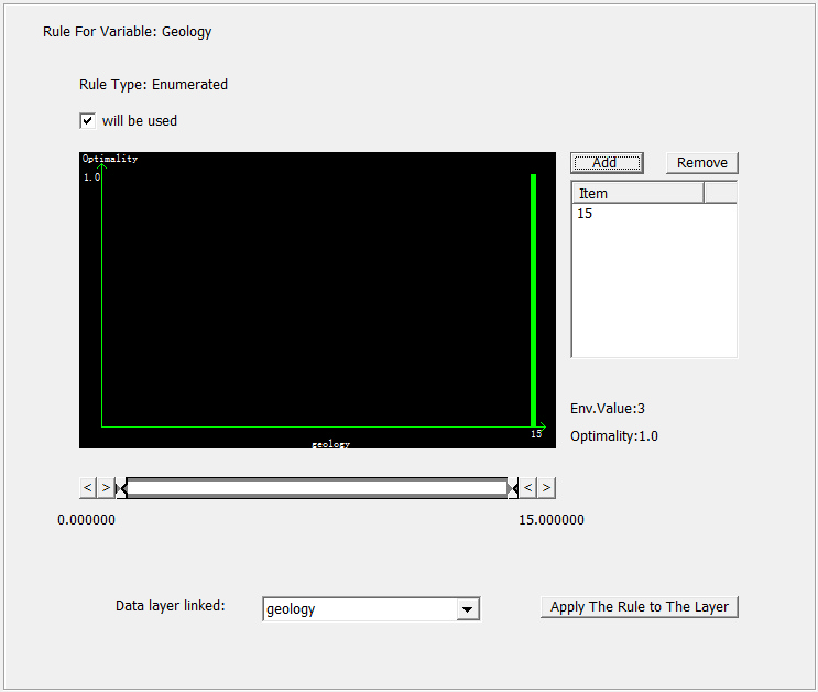
| 5. | In the editing interface, click on "Add". In the pop-up dialog, enter 15. |
A green bar whose x coordinate is 15 will appear in the graphic area and 15 will also be added into the list.
Now we have encoded the knowledge on soil environmental conditions as rules. You can repeat the process for the other soil types.
Save the Project:
Let's save the project through "Project->Save".
The project configuration and knowledge base will be saved into "Test_RuleBased_Project.sip" in the project directory.
At this point your project has been created and saved. You can use the control panel to navigate to the rules that have been created and make changes to them. The next step is to run an inference using the encoded knowledge to produce a soil fuzzy membership map.
Run Inference:
SoLIM Solutions will create a set of soil fuzzy membership maps, one for each soil type which has soil-landscape knowledge defined in the current knowledge base. In this tutorial, we only have the knowledge for one soil type, so there will be only one soil membership map.
Click "Inference" node to unfold it. Under that node, click "Inference", the view will shift to Inference interface.
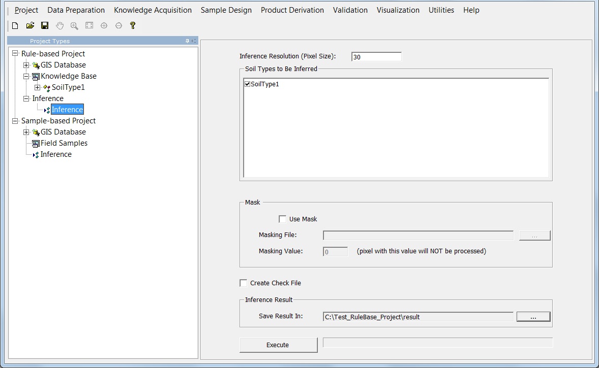
In this view, you can specify the resolution of the inference result . The default resolution is the same as the resolution of the first GIS data layer. We use the default resolution here.
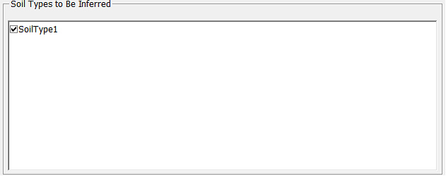
In the "Soil Types to Be Inferred" list, check "SoilType1" to specify that a soil membership map will be created for this soil type.
Uncheck the box next to "Use Mask" so that no mask will be used in this tutorial. The mask is used to limit the area of inference. Inference is only performed over areas with values of 1 in the mask.
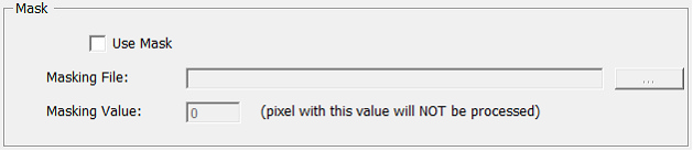
Uncheck the box next to "Create Check File", so no check file will be created. The check file is used to log the information on inference at every location where inference is performed.
![]()
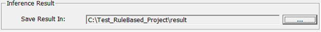
Click on![]() button within the region of "Inference Result", a dialog will appear for you to create or choose output directory.
button within the region of "Inference Result", a dialog will appear for you to create or choose output directory.
Create a results directory "result" in the "Test_RuleBased_Project" directory to host the output membership maps using the "Make New Folder" button.
Click on "OK", the directory will appear on the "Save Result in" text box.
Click on "Execute", in less than a minute a dialog should pop up to inform the completion of the inference. Otherwise, an error message should show up to tell you what was wrong.
Viewing Results:
After the inference has completed, you may want to view the results in graphic form. Inference output consists of one fuzzy membership map in a raster form for each named soil. Each raster is stored in a separate file with name NameID.3dr where ID is the soil identification number (unique to each soil type) and Name is the soil type name. After the tutorial inference is complete, the following file will exist:
SoilType1.3dr
Please examine the relationship between the filename of the output fuzzy membership map and the name used in the knowledge base for the soil type. Be sure that each soil type has a unique ID number.
There are three ways to view the results. One is to convert the 3dr file into GRID ASCII format and view the results in other GIS software, such as ArcGIS (see Untilities->File Converter for details on exporting 3dr file into GRID ASCII format). The second is to use the 3dMapper (available at www.terrainanalytics.com). The third way is to view the results using the Data Viewer provided by SoLIM Solutions 2013. In this tutorial, we will use the 2D Data Viewer to visualize the results.
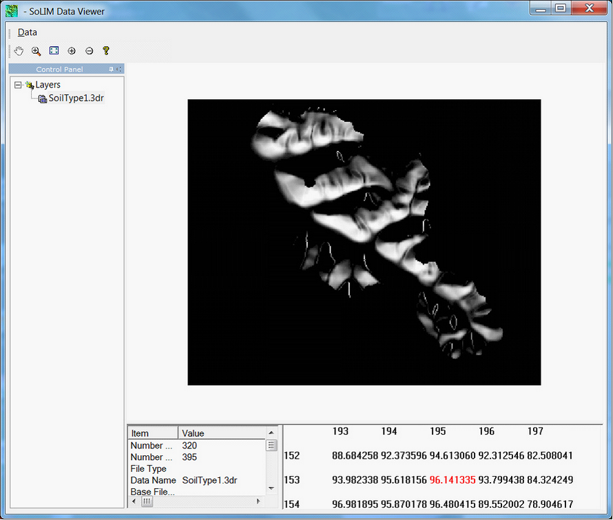
Choose "Visualization->2D" and open the Data Viewer.
Choose Data->Add Layer.
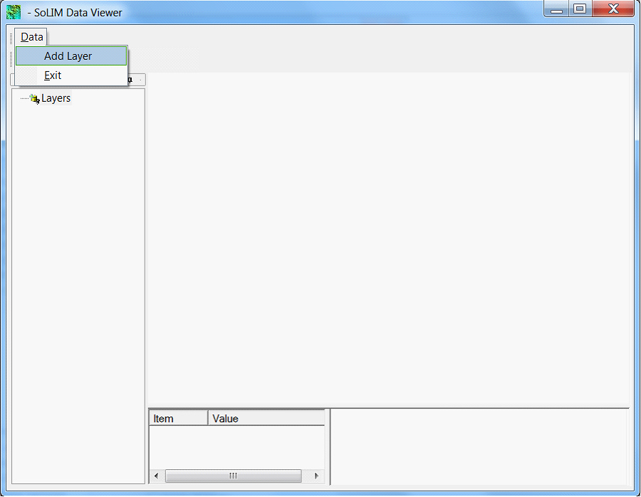
Navigate to the output directory and select SoilType1.3dr to open it. You should now see this new raster data layer is added to the left layer list panel. At the same time, the layer (the fuzzy membership map for soil type 1) is displayed in the graphic area.
You have now learned the basics of soil mapping using rule-base project in SoLIM Solutions 2013. Feel free to play around with the membership functions and examine the impact on the output. As an exercise, you could create another soil with different rules and re-inference. By bringing the new soil's membership map into Data Viewer, you could compare its distribution with SoilType1.